Excel Formula To Pull Non Numeric From Multiple Worksheets

Since you want to be able to pull this formula down fix this cell reference to B4. There are two options The VLOOKUP and CHOOSE function or INDEX and MATCH function both is an array formula.

Tom S Tutorials For Excel One Formula Returns Value Of The Same Cell On Multiple Worksheets Tom Urtis

After locating and clicking OK Excel will enter.

Excel formula to pull non numeric from multiple worksheets. Figure 7 How to merge two Excel Sheets. Since you know that you will be looking at the Game Div. TEXTJOIN TRUE IFERROR MID B5 ROW INDIRECT 1100 1 0.

To remove non-numeric characters from a text string you can use a formula based on the the TEXTJOIN function. ExcelCurrentWorkbook Figure 8 combine excel files. Excel automatically writes the correct address of the data table into the formula.

In the Fill Worksheets References dialog box choose Fill vertically cell after cell from the Fill order and click the little lock beside the formula text box and the grey lock will become yellow lock it means the formula and cell reference has been locked then you can click any a cell to extract the cell B8 references from other worksheets in this example I will click cell B2. Create the named range that lists the names of the worksheets Sheets in the tutorial create a unique list of each employee then the formula would be something like SUMPRODUCTCOUNTIFINDIRECTSheetsA1A10B1. COUNTIFSheet1A2A6D2COUNTIFSheet10A2A6D2COUNTIFSheet15A2A6D2 Sheet1 Sheet10 and Sheet15 are the worksheets that you want to count D2 is the criteria that you based.

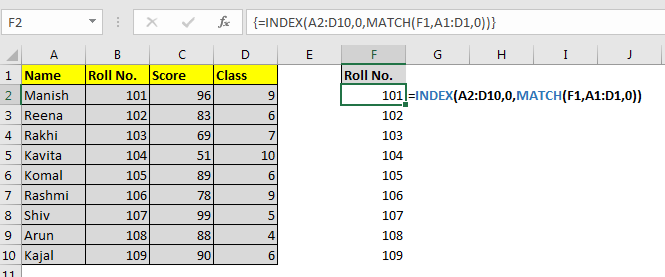
To combine tables we will click on the double pointed arrow in the content header cell. Copying the formula to cell D2 E2 we will get the value of cell A1 from the respective sheets. Lookup value is the cell containing the month cell B4.

This function can be used to count the different kinds of cells with number date text values blank non-blanks or containing specific. In the Editor we will enter the formula below in the formula bar. VLookup can pull email addresses from Spreadsheet 2 into Spreadsheet 1 by matching CampusID 555123123 in both spreadsheets.

Heres how to create a VLOOKUP formula that pulls data from another workbook. While writing the formula select the worksheet that has the correct data table and select the data table. Excel COUNTIF function The Excel COUNTIF function will count the number of cells in a range that meet a given criteria.

Figure 9 merge excel documents. Press Enter on your keyboard. You get all the non numeric characters removed.

For Non-Numeric Result The easiest solution is to use the VLOOKUP function and the helper column. For example we want to add a column for email address but that data exists on a separate spreadsheet. In Excel you can also use the COUNTIF function to add the worksheet one by one please do with the following formula.

We will hit the Enter key to show all table names. Tab this does not need to be an argument. In the example shown the formula in C5 is.

Excels vLookup formula pulls data from one spreadsheet into another by matching on a unique identifier located in both spreadsheets. VLOOKUP lookup_value Sheetrange col_index_num range_lookup. Drag down this formula to remove characters from string from all the cells in column C3.

For example the below formula will multiply numbers by 10 and yield Not number for non-numeric values. To make sure you only get to combine the tables from the worksheet you need to somehow filter only these tables that you want to combine and remove everything else. The generic formula to VLOOKUP from another sheet is as follows.

If a worksheet containing data that you need to consolidate is in another workbook click Browse to locate that workbook. The difference is that you include the sheet name in the table_array argument to tell your formula in which worksheet the lookup range is located. IFISNUMBERA2 A210 Not number Check if a range contains any number.

TEXTJOINTRUEIFERRORMIDC3SEQUENCE2010 And when you hit the enter button. If you want no helper column in the worksheet then you can use the virtual helper column in the formula. Once you insert ExcelCurrentWorkbook in the Power Query formula bar and hit enter you get a list of Excel Tables.

Apply the above generic formula here to strip out the non numeric characters. Click the worksheet that contains the data you want to consolidate select the data and then click the Expand Dialog button on the right to return to the Consolidate dialog. In this way we will find a formula very helpful that will give a value from all the multiple sheets in the workbook.

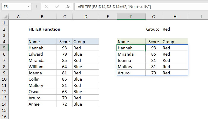
How To Use The Excel Filter Function Exceljet

Excel Vlookup Multiple Sheets My Online Training Hub

How To Limit Number Of Decimal Places In Formula In Excel

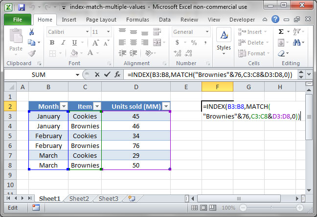
Index Match With Multiple Criteria Deskbright

How To Vlookup Values Across Multiple Worksheets

Excel Formula If Not Blank Multiple Cells Exceljet

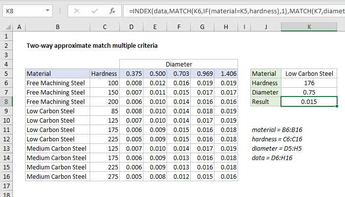
Excel Formula Two Way Approximate Match Multiple Criteria Exceljet

Data Consolidation If You Chose To Link To The Source Data Then Each Cell Will Contain A Formula Linking Back To The Original Data Data Consolidation Excel

How To Use Division Formula In Excel Microsoft Excel Excel Tutorials Microsoft Excel Tutorial

How To Calculate Average Cells From Different Sheets In Excel

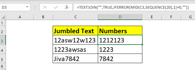
How To Remove Non Numeric Characters From Cells In Excel

Excel Formula Find And Replace Multiple Values Exceljet

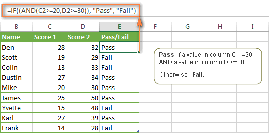
Excel If Statement With Multiple And Or Conditions Nested If Formulas Etc

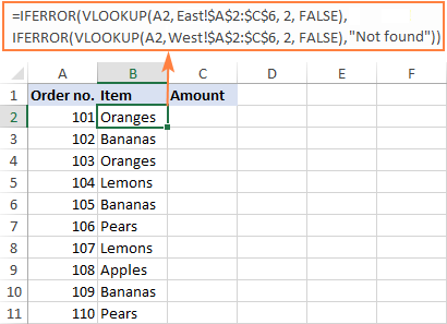
Vlookup Across Multiple Sheets In Excel With Examples

How To Vlookup And Return Multiple Values Vertically In Excel

How To Lookup Entire Column In Excel Using Index Match

Excel Formula Minimum If Multiple Criteria Exceljet

Excel Formula Extract Multiple Matches Into Separate Rows Exceljet

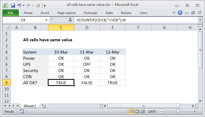
Excel Formula Multiple Cells Have Same Value Exceljet